
Constraints establish limits in optimization models, delineating the feasible region and the location of the optimal solution within that region. Understanding which constraints are impacting the solution and by how much is crucial as it helps identify bottlenecks and limiting factors, providing insights into the critical elements determining the optimal solution.
Constraint Types
Constraints define limits on resources and come in three types:
- Upper bound (<=)
- Lower bound (>=)
- Equality (=)
Regardless of the type, all constraints are composed of:
- Outputs (Left Hand Side – LHS)
- An operator defining the bound,
- A value (Right Hand Side – RHS)
- The periods in which it applies.
| LHS | Bound | RHS | Periods |
|---|---|---|---|
|
oHarvestVolume |
>= |
50000 |
1.._LENGTH |
|
oBudget |
<= |
1000000 |
1.._LENGTH |
|
oBareland |
= |
0 |
_LENGTH |
Binding vs. Non-binding Constraints
A binding constraint is one whose LHS value equals the RHS value in the optimal solution. In other words, the output is at the constraint limit. For example, in the constraints above, if the budget equals 1,000,000 in any period it is a binding constraint. Binding constraints limit the optimal solution and so changing a binding constraint will necessarily change the optimal solution.
Conversely, a non-binding constraint is one whose LHS value does not equal the RHS value in the optimal solution. There is room to spare, or excess capacity in the system. Removing a non-binding constraint will not change the optimal solution all other things being equal.
Shadow Prices
A shadow price is the marginal cost of a constraint in units of the objective function, indicating how much the objective function changes if the RHS value increases by one unit.
- Positive Shadow Price: The objective function value will increase.
- Negative Shadow Price: The objective function value will decrease.
- Zero Shadow Price: The constraint is not limiting the optimal solution.
Shadow prices provide a tangible value or cost to constraints, allowing for comparison on an equal footing.
Piecing It All Together
How do you determine which constraints are binding, and of those which ones are impacting the optimal solution most?
Woodstock provides a constraint report listing constraints, their binding status, and shadow prices.
Here’s how you set it up:
- Declare a constraint report in your model’s Reports section:
*TARGET Constraints.dbf
_CONSTRAINTREPORT 1.._LENGTH - Compile your scenario to create the report. You must generate and solve your model to generate the shadow price data for the report. Thereafter, you need only compile the model.
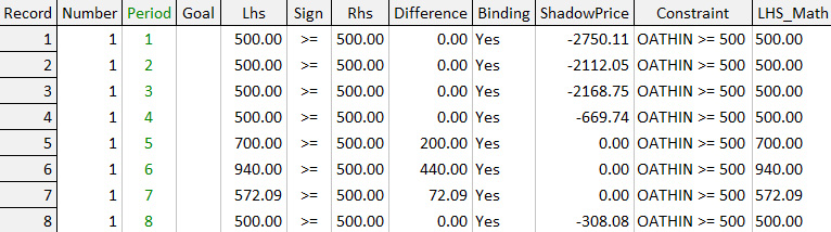
The report contains the following information:
- Number: Order of the constraint in the Optimize section.
- Period: Time period for the constraint.
- Goal: Name and penalty for goal-related constraints.
- LHS: Value of output in the optimal solution.
- Sign: Whether the constraint is <=, >=, or =.
- RHS: The value defining the constraint limit.
- Difference: The difference between the LHS and the RHS value.
- Binding: “Yes” if constraint at its RHS bound in a period (i.e., Difference = 0).
- Shadow Price: The shadow price (not available for MIP/IP models).
- Constraint: The constraint as declared in Optimize section.
- LHS_Math: Breakdown of how the LHS was calculated.
How are Shadow Prices and Binding Constraints Calculated?
Shadow prices are calculated by the solver as part of the solution. Binding status is calculated by Woodstock by comparing the LHS and RHS value of the constraint. If the values are equal in even one period, the constraint is binding.
Shadow prices do not influence the binding status. Even in MIP models that do not calculate shadow prices, the report identifies binding and non-binding constraints.
Example and Practical Tips
Example:
The report snippet above was generated in a discounted cash flow model maximizing net present value subject to a lower bound constraint on the area thinned. The constraint is binding because the LHS value equals the RHS value in a period.
How costly is the constraint? The shadow price indicates that in period one, the constraint cost -2,750 units of net present value. This means that if the RHS value is increased by one unit, the net present value will decrease by 2,750.
Practical Tips
- Look for binding constraints: These are the constraints where the LHS equals the RHS in a period.
- Focus on large shadow prices: Constraints with larger shadow prices have a more significant impact on the solution.
- Understand non-binding constraints: If a constraint is not binding and has a shadow price of zero, it’s not affecting the solution. However, it may become relevant if the model changes.
FAQ
How do I identify the most restrictive constraint in my model?
Binding constraints limit the optimal solution, and shadow prices indicate the cost. For binding constraints, the larger the shadow price, the more restrictive it is.
Can I remove non-binding constraints?
Non-binding constraints can be removed, but the outputs should be monitored. If the model changes, a non-binding constraint may become binding. Small deviations from the intended constraint RHS value may be acceptable, but it is up to you to determine if the solution is acceptable without the constraint.
Read more in the Woodstock Documentation System.
- Sensitivity analysis: Understanding reduced costs and shadow prices (ID 1358)
- How do I know what constraints are binding (ID 3090)
- A recipe for understanding linear programming (ID 1402)
- Finding an optimal solution (ID 347)